


Rendering a Buddhabrot at 4K and Other Bad Ideas
Recently I have been digging through some old projects and rediscovered an old high school project of mine that attempted to render very large images of the Buddhabrot fractal. I did not know a lot about writing fast code back then, and unsurprisingly that project was unsuccessful. However, I don't like leaving things unfinished, and for the past few months I have been writing a modern GPU implementation of a Buddhabrot renderer to see where I could take it.
Instead of rendering a single large image, I thought an animation sequence would be more interesting to look at. The Buddhabrot lives in a 4D space, and rotating through different projections onto a 2D screen does better justice to its intricate shapes. However, feature creep set in, and this ended up being a lot more complex to do than originally intended - a single camera pan was not interesting enough, and I started writing a lot of throw-away tools to setup 4D camera shots synchronized to music. I was also set on rendering at 4K resolution, and render times shot through the roof. A lot of time went into careful importance sampling code and denoising methods to keep render costs in check.
Programming and camera setup took the better of two months, and rendering the final animation took more than 10 days. My poor GTX480 also ended up dying a fiery death at the hands of the fractal, and I had to borrow a computer to finish the job. I am not convinced it was worth it, but I'm happy to finally put the project to rest :)
A Buddhawhat?
The Buddhabrot is a curious fractal that produces wonderful images of cloudy and colorful nebulas, and is closely related to the Mandelbrot set. The Wikipedia pages on the Mandelbrot and the Buddhabrot are a better resource, but briefly, the Mandelbrot set works by picking points on the complex plane, repeatedly transforming them with a simple formula and checking whether the points eventually escape outwards to infinity or not. The points that do not escape become part of the set.
The Mandelbrot fractal is fascinating, because it generates a point set of mind-boggling complexity from a few very simple rules. This emergent complexity seems to be a funky property of the complex plane, and many other fractals have been made using similarly simple rules over the complex numbers. One such fractal is the Buddhabrot.
The Buddhabrot uses the same iteration rules as the Mandelbrot: Points are sampled on the complex plane, repeatedly transformed using a simple function, and filtered based on whether they escape to infinity or not. The major difference, however, is which points are kept: If a point does not escape, it is thrown away; but if it does escape, the point and all of its transformed versions are stored. The transformed versions of the point correspond to its "trajectory" through space as it escapes to infinity.
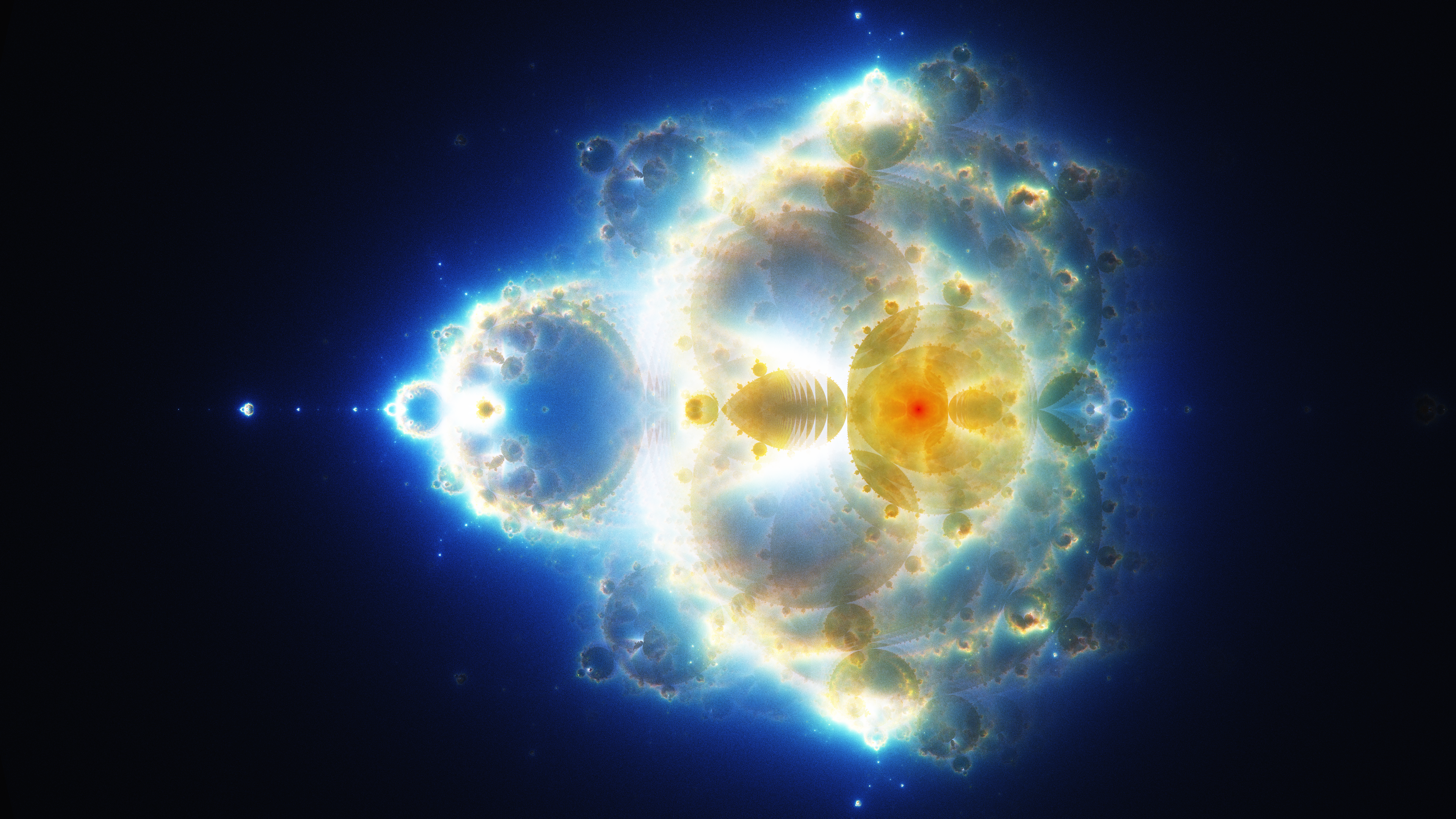
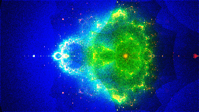
If we do this many times, we will end up with a large list of points not in the Mandelbrot set and their trajectories on their way to infinity. To obtain a Buddhabrot, we simply build an image representing a histogram of these trajectories: We start with a black image, and whenever a trajectory passes through a pixel, we increment it by one. If we keep doing this, we will eventually obtain an image where bright pixels show regions that are visited often by escape trajectories, and dark pixels to those visited rarely. This is the Buddhabrot.
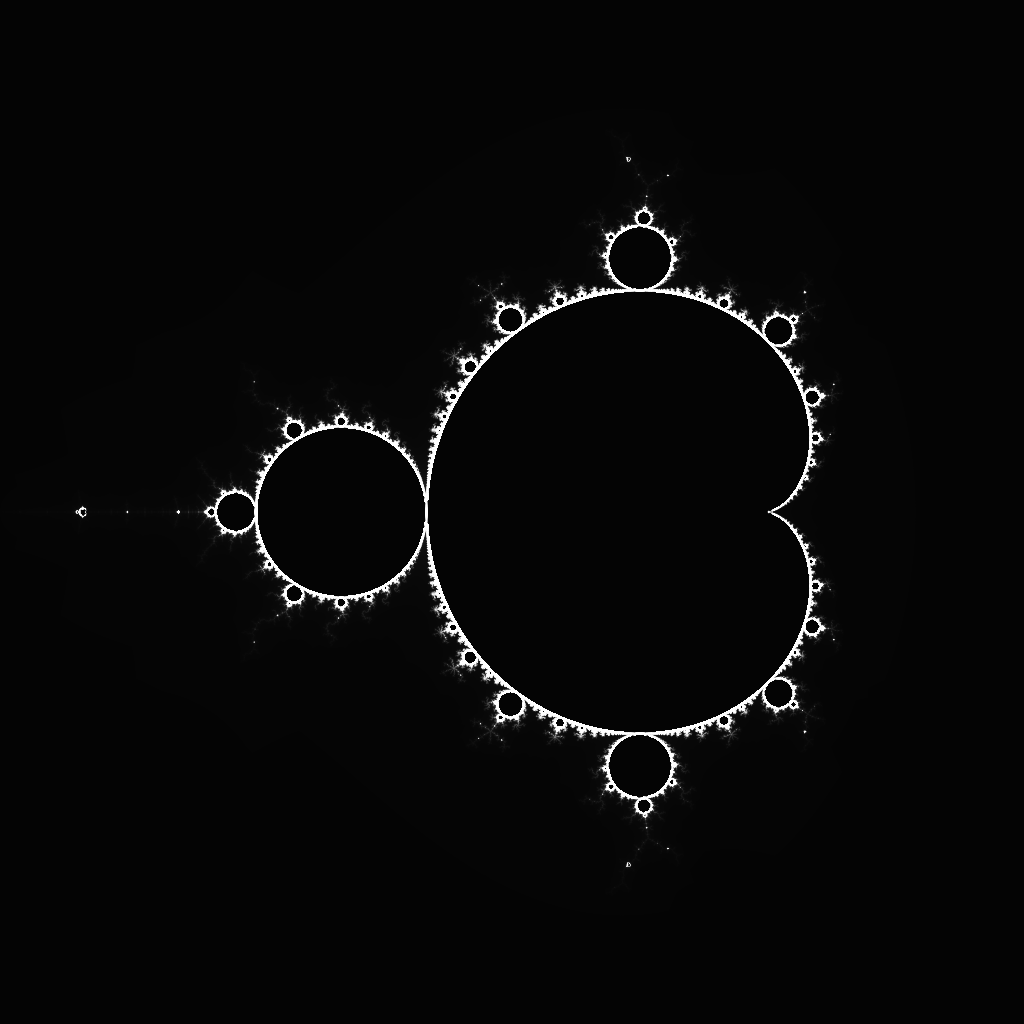
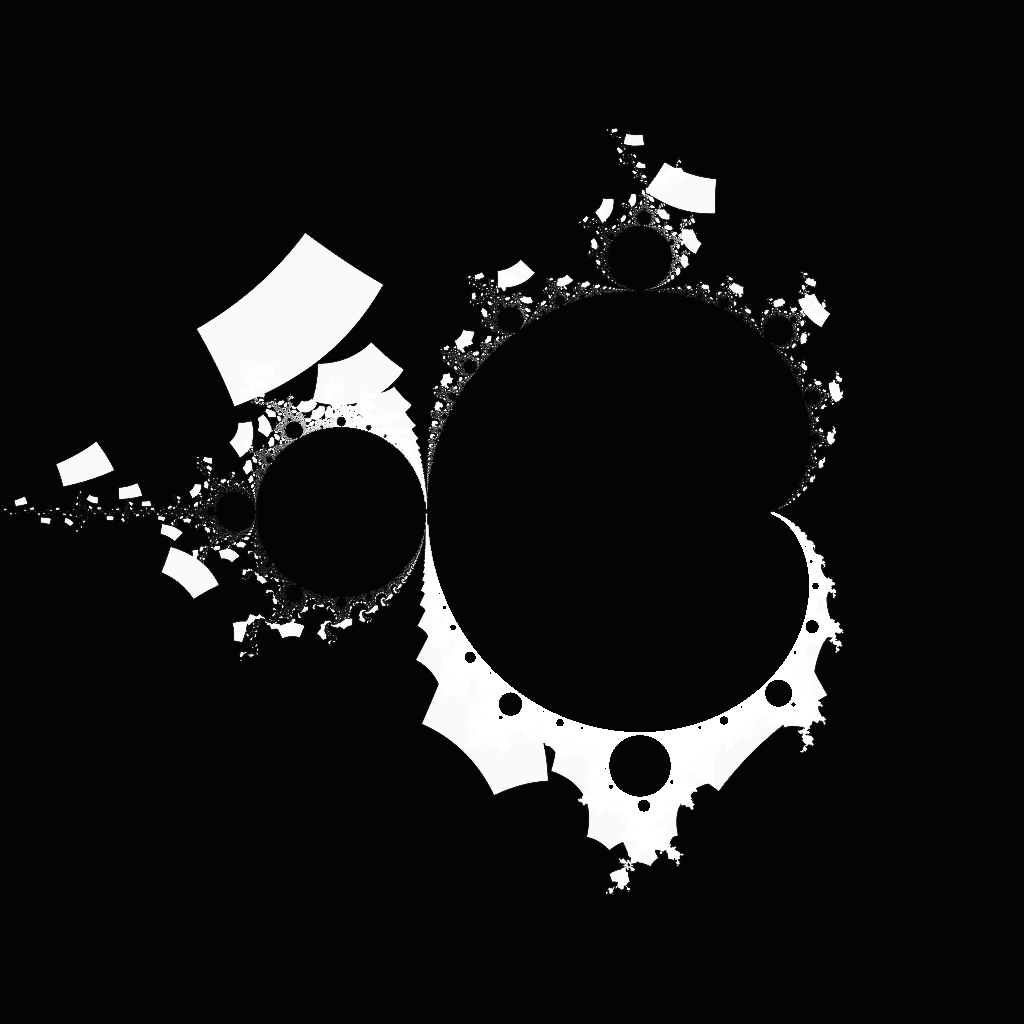
How to map trajectories to pixels is a matter of projection, and Melinda Green (the discoverer of the Buddhabrot) has more resources on the topic. Interestingly, the Buddhabrot contains the entirety of the Mandelbrot, and with the right projections we can rotate back and forth between the two.
Rotating between the Buddhabrot and the Mandelbrot fractal
Importance sampling
Rendering the Buddhabrot efficiently poses a bit of a challenge. The main problem is that we cannot directly compute the value of the Buddhabrot at a pixel, but have to sample many random trajectories and hope that they pass through the pixels we care about. This "spray and pray" approach works reasonably well for zoomed out images, but zoom-ins and transformations are very difficult to render in a reasonable time frame, since many trajectories land outside the frame and their computation is wasted.
However, if we're a bit smarter about how we sample the starting points of the trajectories, we can mitigate this problem. Trajectories are completely determined by their starting point, and the usefulness of a trajectory is determined by how many histogram bins it touches before escaping. Long trajectories inside the frame are much better than short trajectories or trajectories completely off-screen. We can therefore rate each starting point by an importance value, which is equal to how many bins it touched before escaping.
We don't know the importance distribution a priori, and initially we have no choice but to sample starting points uniformly random. However, if we record the importance values of the generated points in a separate importance image, over time we start getting a good idea of which areas tend to contain starting points that produce important trajectories, and which areas are irrelevant for the region we are rendering.
The image below demonstrates the importance map (right image) for rendering a zoomed out Buddhabrot. Note that the importance map is almost equivalent to an image of the Mandelbrot set: Important trajectories almost all start right at the border of the Mandelbrot set.

The Buddhabrot (left) and its estimated importance map for generating trajectories (right). Note that the importance map corresponds to the Mandelbrot fractal.
Things start looking a little bit more interesting for zoomed in versions. Important points now tend to come from the lower half of the Mandelbrot set, but warped rectangular pools of important points are distributed all over.

A zoomed version of the Buddhabrot (left) and the estimated importance map for generating trajectories (right).
After generating a decently converged importance map, we can apply standard 2D Monte Carlo importance sampling to draw samples from it. Instead of generating trajectories uniformly random, we pick their starting points such that we start off trajectories more often in regions which we think contain many important points. In zoomed out images, this sampling strategy already creates some impressive speedups, and zoom-ins benefit immensely from this method.
It's worth noting that we need to change the weights of the trajectories accordingly - instead of incrementing histogram bins by one, we need to increment them by the inverse probability of sampling a trajectory. This corresponds to the standard Monte Carlo estimator.
I should mention that Alexander Boswell discovered a similar sampling technique. He uses the same importance function, but rather than representing it explicitly and sampling it using a 2D map, he uses the Metropolis-Hastings algorithm to draw samples from it. While this works, Metropolis-Hastings has the drawback that the samples that it generates are correlated. This manifests as "splotchy" noise, rather than white noise, in the image, and poses huge problems in animation. Additionally, as visible above, the importance function can be quite complex with large, black regions, and it is difficult for Metropolis-Hastings to explore it properly. Since the input domain is 2D, we can afford to keep track the importance map explicitly, and in my case this method was better suited than Metropolis-Hastings.
Variance Estimation and Denoising
Importance sampling takes us a long way towards cutting render times for still images. However, animations are an entirely different beast: Decently sized animations need thousands of images, not just one, and we don't have enough time to render each image to convergence even with clever sampling. Additionally, video compression mixes very poorly with noisy data, and noisy video becomes almost unusable after Youtube is done with it. Somehow, we need to turn noisy images into something we can work with, without spending more render time on them.
To solve this issue, I turned to literature in the search for a denoising algorithm that would work with Monte Carlo noise. Luckily, this is something the movie industry has dealt with before, and there is plenty of literature on the topic. For this particular project, I chose a Non-Local Means denoising method based on Rouselle et al.'s work in Robust Denoising using Feature and Color Information.

An image generated from one billion trajectories is still too noisy for animation (left). After Non-Local Means denoising, image quality sufficient for 4K video (right).
Non-Local Means is a bit like a very selective blur. It will search neighborhoods of pixels and blend pixels together which it thinks are similar, but will leave pixels alone that are very different. The difference measure here is based on patch-wise distances, which tend to be very robust in practice and allow us to inject additional info about the noise in the image.
To operate effectively, Non-Local Means needs an estimate of the variance at each pixel. The variance measures how noisy a pixel is, and this will make the denoiser be more careful with pixels that are nearly converged, but more aggressive with pixels that are very noisy.
Computing the variance of the Buddhabrot directly is a bit tricky because of the histogram approach. To get a robust estimate, I used a multi-buffer method: Instead of one histogram, the renderer keeps track of multiple histograms at once. When we trace a trajectory, we splat it only to one of the histograms. At the end of the render, this gives us multiple statistically independent renderings of the same scene. Averaging these histograms produces the normal output image, and taking the sample variance across all histograms gives an estimate of the variance.
A rendering of the Buddhabrot (left) after one billion trajectories and the estimated variance at each pixel (right).
For still images, this already gives good results. However, for animations, there is an additional issue of temporal coherence. Monte Carlo generates white noise, which is noise equally distributed over all frequencies. Non-Local Means operates within a finite spatial filter window (here, 31x31 pixels), and can therefore only remove high- to mid frequency noise. Low frequency noise is left behind.
In still images, this is not a huge deal, since human vision is not great at recognizing spatial low frequency variations in brightness. However, this is different in animations: Each frame has a different noise pattern, and the low frequency noise changes in each frame. This cause entire regions in the image to jump up and down in brightness over time, which looks terrible and consumes significant video bandwidth.
To deal with this problem, I implemented a temporal extension of the Non-Local Means filter. In addition to the current image, the previous 5 and the next 5 frames in the animation sequence are also used to help denoise the current image. We not only search similar pixel neighbors in space, but in time as well (this sounds fancier than it is). On the one hand, this further helps remove spatial noise. On the other hand, this smooths out the noise pattern over multiple frames, making the temporal artifacts a lot less apparent.
Standard Non-Local Means denoising (left) leaves behind disturbing low-frequency noise. Temporal Non-Local Means denoising (right) smooths out noise across frames and greatly reduces this problem.
Relation to the Jacobian
Interestingly, the Buddhabrot is intimately related to the inverse Jacobian determinant of the Mandelbrot iteration, and I initially investigated this relation in search for a more efficient rendering algorithm. While I did find an alternative rendering method, it is a lot noisier at high iteration counts and not really feasible. However, I still thought it was interesting, so I will briefly summarize it here.
A crude description of the inverse Jacobian determinant of a function is that it is a measure of how a function stretches and squeezes the space it operates on. The value of the inverse is large where the function compresses the input space, and small where it stretches it.
The Mandelbrot iteration itself is a series of functions from the complex plane to the complex plane. For example, iterating a point once, iterating a point twice and iterating it three times are three different (polynomial) functions that transform complex points to other complex points. For the Mandelbrot, these functions are usually not given explicitly, but are written down as a recursive rule; however, if we keep expanding and multiply out the terms we eventually arrive at a simple polynomial function for each iteration.
We can compute the inverse Jacobian determinant of these functions to figure out how they compress and stretch the complex plane. If we do this for each iteration of the Mandelbrot and sum the inverse determinants of all of these Jacobians, we get a new function that measures how space around a point gets distorted as it is run through the Mandelbrot iteration. The Buddhabrot computes exactly this function.
The Jacobian of the Mandelbrot iteration can be derived analytically. To arrive at an alternative rendering method, instead of counting the number of trajectories that pass through a pixel, we can instead compute the average Jacobian determinant of all trajectories passing through a pixel. After rendering, we take the inverse of each pixel value, computing the inverse average Jacobian determinant.
This will generate exactly the same Buddhabrot as the histogram approach, up to a global scaling factor. Initially I was hoping this to be vastly more efficient than the histogram approach, and for low iteration counts this is the case. However, the inversion at the end greatly inflates the variance at higher iteration counts, and this approach ends up being a lot less efficient than the standard histogram.